
· performance
Building and Testing Galactus, My Local LLM Server
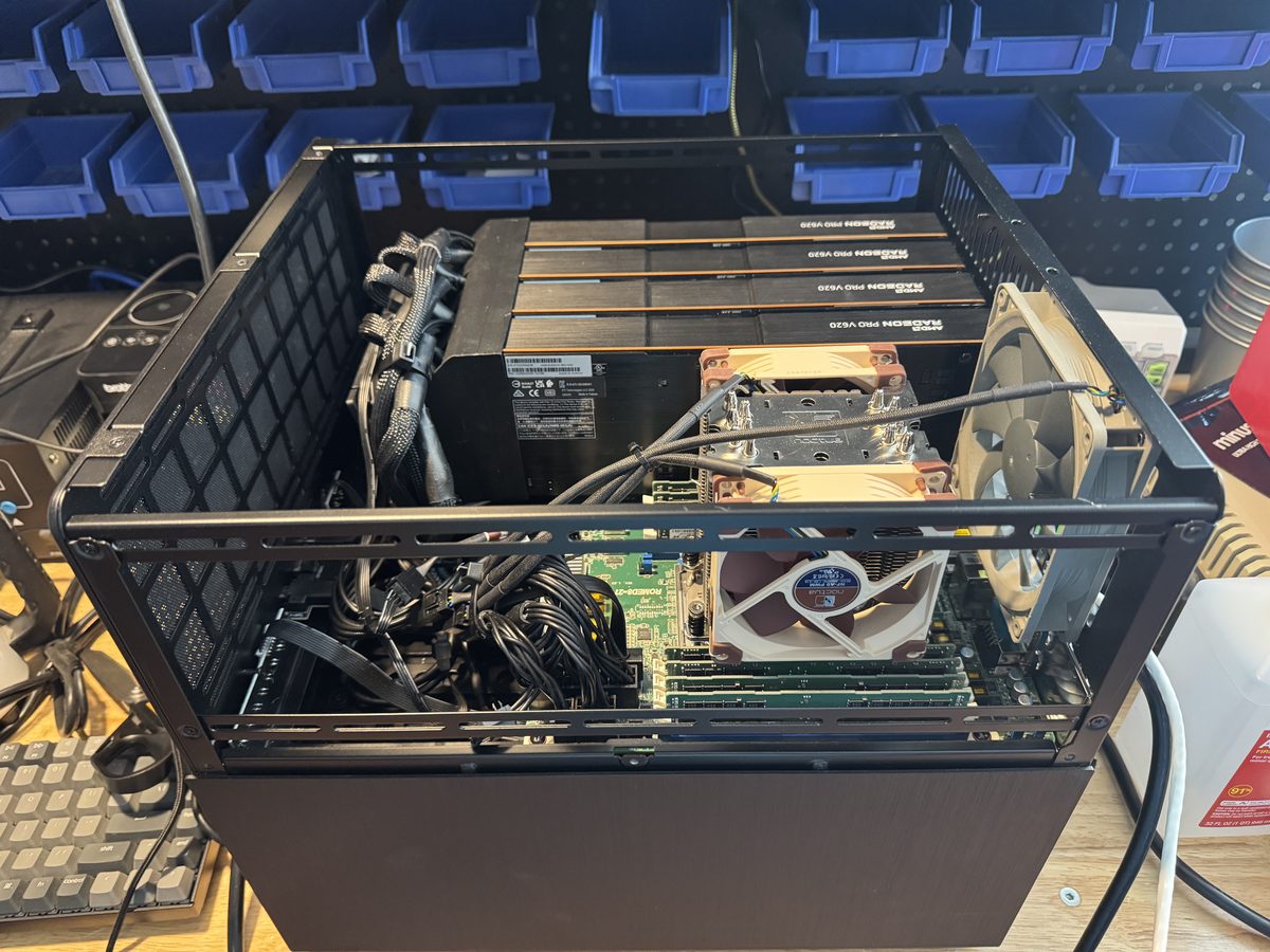
Update: This account covers the initial setup, the July investigation with 1 TB of RAM, and the August expansion to 2 TB. The model lineup and llama.cpp build have changed since these tests. The performance-engineering notebook retains the later measurements and exact configurations.
I built Galactus to run open-weight models whose memory requirements exceed those of a conventional GPU workstation. The initial targets included Kimi K2.5 and Qwen 3.5 397B; later, GLM-5.2 provided a particularly demanding test, with a roughly 435 GiB quantized export. Holding that much model data entirely in GPU memory would have required a very different budget.
The design combines a large bank of system RAM with four smaller GPU memory banks. That made the models fit, but fitting was only the first requirement. I also needed to establish whether the machine could generate text at a useful rate, process a substantial prompt, and expose enough control over placement to use the hardware I had bought.
Choosing the memory and GPUs
These models use a mixture-of-experts architecture. Their full expert bank occupies a great deal of memory, while each generated token selects only a subset of those experts. Total model size determines the capacity required to load it; the selected weights and the operations around them help determine how quickly it runs.
I chose the AMD EPYC 7713 for its eight memory channels. It has 64 physical cores and 128 hardware threads, but the memory channels were more relevant to the intended workload than the prospect of using every thread. With many expert weights in system RAM, generation repeatedly reads those weights through the host’s memory system.
The GPUs were surplus Radeon Pro V620s that I found on eBay for $400 each. Four cards cost $1,600 and supplied 128 GB of nominal aggregate VRAM, reported by the runtime as roughly 120 GiB. This was enough to hold attention and other always-used tensors, plus some resident experts where the chosen configuration allowed it, while the larger routed-expert bank remained in system RAM.
The main components and the memory changes were:
| Component | Configuration |
|---|---|
| CPU | AMD EPYC 7713, 64 cores / 128 threads |
| July system RAM | 8 × 128 GB ECC RDIMMs, 1 TB total, configured at 2933 MT/s |
| August system RAM | 8 × 256 GB DDR4-2933 3DS RDIMMs, 2 TB total |
| GPUs | 4 × Radeon Pro V620, 32 GB nominal VRAM per card |
| Chassis | Jonsbo N5 |
| Inference stack | llama.cpp with ROCm, inside an LXC container on Proxmox |
The passive V620s also needed cooling suitable for this chassis. I used custom 3D-printed fan shrouds with high-static-pressure server fans to direct air through the cards.
The original 1 TB build cost about $9,050, with the following amounts recorded in July:
| Component | Recorded cost |
|---|---|
| 1 TB of RAM | $5,600 |
| Four V620 GPUs, including tax and shipping | $1,600 |
| EPYC 7713 CPU | $600 |
| Motherboard | $600 |
| Power supply | $400 |
| Case | $250 |
| Total | $9,050 |
RAM and the GPUs consumed most of that budget. The replacement 2 TB DIMM population cost $7,800 in August. These are historical costs for my build; the recorded total does not separately itemize storage, cooling, or accessories.
Getting the software stack working
I used Proxmox for the host and ran inference in an unprivileged Debian LXC container. The same host also handles storage and networking. Open WebUI supplied the inference interface, with llama-server providing an OpenAI-compatible endpoint. The March setup notes record two integration problems that had to be resolved before model throughput was meaningful.
First, the container setup exposed the GPUs’ render devices but omitted /dev/kfd, which ROCm also needed in this installation. Correcting device access made the cards usable from the container. The workaround is retained in the build notes as part of that installation’s history; it is not a complete template for configuring device permissions on another host.
Second, compiling llama.cpp with Debian’s system compiler failed because it could not read the device bitcode supplied by the installed ROCm toolchain. Pointing the build at ROCm’s bundled clang resolved that mismatch. The working build enabled the HIP backend and targeted gfx1030, the V620’s architecture identifier.
Later platform checks compared STREAM bandwidth on the host and inside the container. The results agreed within about 1–2%, and the July cgroups had no CPU or memory throttling limits. That supported using the container for the memory-intensive tests; it did not measure every possible cost of the software stack. The early March container had its own resource ceilings, so its timings cannot be treated as equivalent to the later unrestricted configuration.
A memory upgrade that changed the machine’s behavior
The early memory population mixed four 128 GB DIMMs with four 64 GB DIMMs. In the March record, this configuration reached only about 30 GB/s in the large STREAM test. Replacing it with eight matched 128 GB DIMMs produced 141 GB/s in STREAM Copy and 107 GB/s in Triad.
On the same recorded Qwen Q4 placement, generation increased from 8.5 to 12.4–12.7 tokens/s after the DIMM replacement. This was an important improvement in the workload I actually wanted to run. The bandwidth result rose much more than generation throughput because generation includes computation and synchronization as well as memory reads.
The comparison supports the DIMM replacement as a useful change, but it does not identify the exact reason the mixed population performed so poorly. The original interleaving explanation was not verified against the controller’s address mapping. I therefore keep the observed improvement separate from that proposed mechanism.
The July thread sweep later produced rates that, after the stated write-traffic adjustments, clustered around 152 GB/s. Those adjusted estimates differ from the raw March Copy and Triad rates, so the figures should not be read as one continuous bandwidth series. They did give me a practical reference for the memory path used in the GLM investigation.
In August I installed eight 256 GB DIMMs, bringing capacity to 2 TB. One DIMM failed and was replaced on August 15. The subsequent bandwidth check produced adjusted rates around 148–151 GB/s, close to the July reference. For this build, the expansion supplied substantially more capacity without a large change in measured streaming bandwidth. The hardware record retains the separate populations and captures.
What the GPU capacity could actually hold
The March Qwen tests used explicit tensor placement to spread selected expert layers across the four cards. A Q6 export generated about 4.4 tokens/s with the expert bank on the CPU and 5.5 tokens/s with 16 expert layers placed on the GPUs. Moving to a smaller Q4 export allowed 24 expert layers to fit and reached 8.5 tokens/s before the DIMM replacement.
The Q4 comparison changed quantization and placement together, so it does not isolate the benefit of either. It does show how model size and GPU residency interact: smaller expert tensors can free room for more layers, reducing the expert bank served from host memory.
The four cards have separate allocation limits, so placement required checking each one. In these trials, ROCm0 carried a substantial compute-buffer allocation, and an attempt to put eight expert layers there failed with an out-of-memory error. Dividing total VRAM by the size of an expert layer would have missed that constraint. Larger context allocations and wider microbatches also competed with resident weights for space.
The March production configuration reached 12.4–12.7 tokens/s with a 16K context allocation after the matched-DIMM change. This was a usable result for that Qwen export and placement.
Testing model loading and prompt processing
Loading a large model was a substantial part of using the machine. In one July GLM run, the first memory-mapped load took roughly 25 minutes, while subsequent warm loads took about 45–90 seconds. Those timings belong to that storage and cache state, but they show why generation throughput alone does not describe the experience of switching models.
July GLM-5.2 decode rates were around 5.5 tokens/s with experts in system RAM, or 6.01 tokens/s when the fitter placed some expert layers on the GPUs. Prompt processing needed a separate investigation.
An early benchmark script left the prompt at 512 tokens while requesting larger microbatches. llama-bench capped the effective microbatch at the prompt length, so those runs never exercised the intended large-batch configuration. With an 8192-token prompt held constant, increasing the microbatch from 512 to 8192 raised prefill from 25.90 to 104.97 tokens/s. The useful lesson for testing this build was to check what the engine actually ran, rather than relying on the requested flags.
The scheduler investigation then found an uneven assignment of GPU work and a routing readback that could delay subsequent transfers. Distributing the work alone measured 105.71 tokens/s, little improvement over stock. Combining distribution with a large-batch readback bypass reached 119.36 tokens/s, a 13.7% gain over 104.97. At that rate, the measured 8192-token prefill pass took about 69 seconds.
This patch improved a particular prefill path. The patch record contains the code, attribution checks, and conditions under which I measured the gain.
What the later tests achieved
After the RAM replacement, I measured a common baseline on August 15–16 using llama.cpp build 3653e6d6d, the stock scheduler, and CPU-resident routed experts. Prompt length and microbatch were both 8192, with generation measured over 128 tokens. GLM used 32 threads; the other models used 64.
| Model | Prefill at 8192 tokens (tokens/s) | Ordinary decode (tokens/s) |
|---|---|---|
| MiniMax M2.7 | 418.83 ± 24.11 | 15.18 ± 0.18 |
| Qwen 3.5 397B | 249.61 ± 19.78 | 9.37 ± 0.16 |
| DeepSeek-V4-Flash-0731 | 143.54 ± 1.64 | 10.34 ± 0.10 |
| GLM-5.2 | 95.99 ± 3.36 | 5.30 ± 0.00 |
| Kimi K2.6 | 94.23 ± 4.45 | 5.79 ± 0.01 |
The table preserves llama-bench’s reported means and standard deviations from two repetitions. The common-baseline entry identifies the exports and exact commands. Model architecture and quantization differ between rows, so these are the build’s results for those configurations, not a comparison of model quality or an isolated architectural effect.
The July patched GLM result of 119.36 tokens/s belongs to a different build and configuration from the August stock result of 95.99. The lower August rate does not measure a regression caused by the RAM upgrade. Likewise, March’s partly GPU-resident Qwen configuration cannot be compared directly with the August CPU-expert baseline.
On the August build, separate CLI speculation trials reached 6.6 ± 0.3 tokens/s for GLM with MTP and 14.1 ± 0.7 tokens/s for DeepSeek with DSpark. Those trials used a technical prompt and greedy decoding, and repeated timings varied by about 9%. They support useful configurations for that workload, while the benchmark decode column above remains a different test.
What I got from the build
Galactus met the capacity objective: it can load and run models occupying hundreds of gigabytes while using a much smaller GPU memory tier. Its practical speed varies considerably by model, quantization, placement, and phase. A model that fits can still take more than a minute to process a long prompt or generate at only five to six tokens per second. The notebook records what each configuration achieved as the models and software changed.